how to use vlookup

how to use vlookup

VLOOKUP is a powerful Excel function that allows you to look for a specified value in one column of data inside a table, and then fetch a value from another column in the same row.

An example where VLOOKUP might be useful is if you have a monthly sales report in Excel, and want to find the sales made by a specific salesperson from within a monthly sales report. You would lookup the the person's name in the Salesperson column, and then look in the Sales column to find that person's sales for the month.

In this lesson you'll learn how to use VLOOKUP in your spreadsheets. We'll take you through several simple examples where you can see VLOOKUP in action.


STEP 1
First, click into cell D2 – as this is where we want the first vlookup result to appear.
STEP 2
Click on the ‘fx’ button above column B – many people start by typing “=vlookup…” but you don’t have to! Clicking the “fx” button is much quicker!
(you will see the ‘Insert Function’ table pop up – screenshot below)



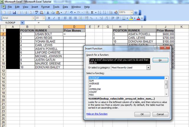
From this window, we will select the vlookup function, as it is one of the ‘most recently used’ functions in the category here.

If the vlookup function isn’t one of the ‘most recently used’ functions, then change the “Or Select a Category” field to ‘All, then scroll to the bottom, where you will see the word ‘vlookup’ and click on it.





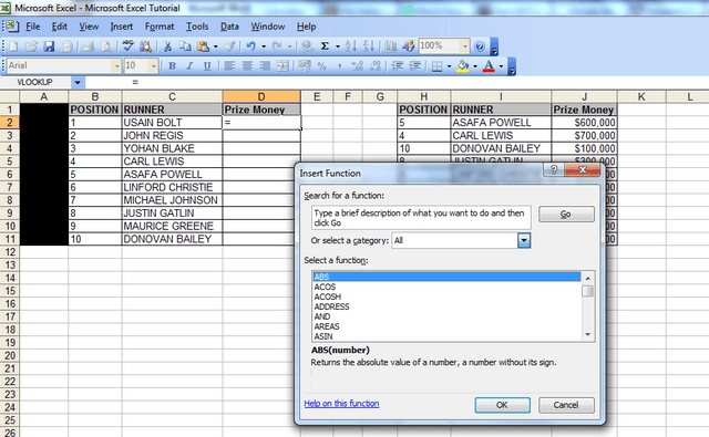
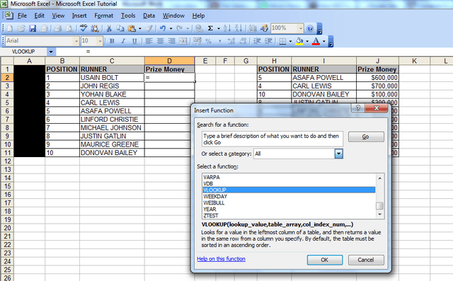
Click ‘ok’ and the function arguments window will pop up. This table will show the Syntax (a fancy word for the format of the formula) and it will display the different parts of the syntax ie

VLOOKUP(lookup_value,table_array,col_index_num,range_lookup)
STEP 3
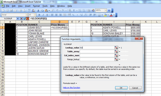
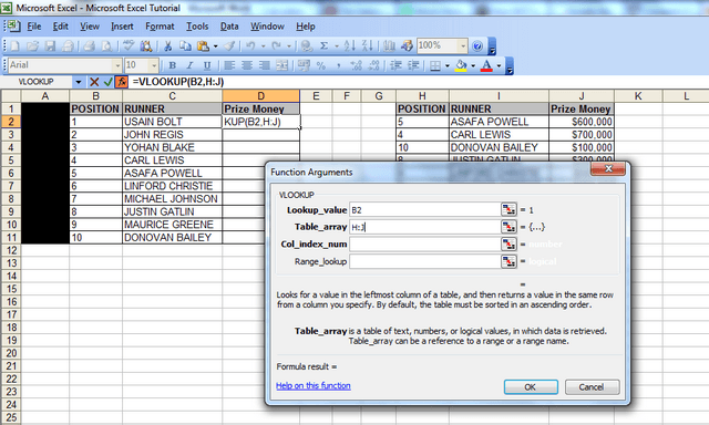
Here, you should click into cell ‘B2’ because that’s the first number or reference for which you want to lookup a value. The ‘look up value’ is the corresponding value we want to find in the first column of the second table – so we want to find out what ‘Prize Money’ the runner in position 1 got in the table that spans columns H to J.



STEP 4
Now click in the next field, the ‘table array’ field (the table array consists of two or more columns of data and the first column in the table array – in this case col. H – has the corresponding numbers that the ‘lookup value is looking at ie the runner positions in this case).
STEP 5
After clicking in the ‘table array’ field, you then need to highlight the columns that that you want to look up data from; so here, we will highlight columns H to J, because our lookup value column starts from column H in the second table, and the Prize Money which we want to check is in col. J
An alternative way to populate the “Table_array” field is to highlight the range of data you’re looking up, starting with your first unique value – in this case cell H2. So you’d highlight cells H2 to J11, because J11 is the last cell in the range. You’d then need to FIX this table array by putting dollar signs in before the H, before the 2, before the J and before the 11, so your formula at the end looks like this: =VLOOKUP(B2,$H$2:$J$11,3,FALSE). If you’re in the table array field and you press F4, then Excel will do this automatically for you. This is useful to know if the spreadsheet doesn’t allow you to highlight cells H to J because some cells are merged or you’re getting an invalid error. But for now, just leave it, ensure, you’re fields look the same as those in the screenshot above then proceed to Step 6, the second last step.



STEP 6
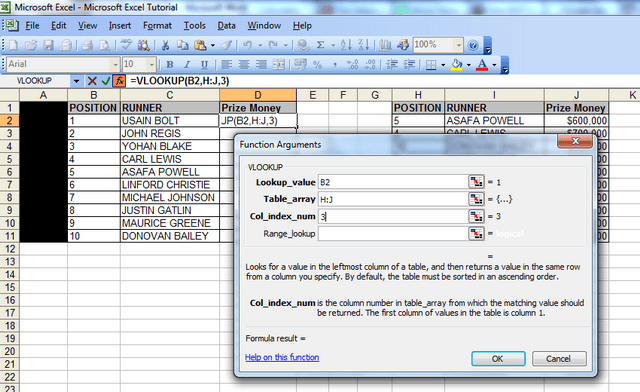
When you highlight the columns, you should note that column J is the 3^rd column from column H. We then move onto the next step, Col_index_num, which is the column Index number. Click in that field and type the number 3) – this is because column J is three columns away from column H.



STEP 7
Now, for the last bit, simply click in the ‘range lookup’ field and type in the word false. You should always type in the word false here, because we want the vlookup to return an exact match for what we‘re looking for, and if it doesn’t then we want it to return the word false.



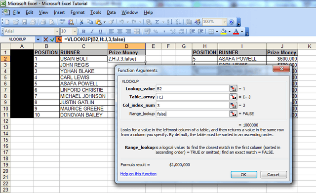
Now click ‘Ok’, and like magic, you will notice that the vlookup has returned the figure of $1,000,000 against Usain Bolt’s name in the first table. If you look at the second table, the figure of $1,000,000 is also against Usain Bolt’s name, so we know the vlookup has worked. And that’s how you string together the vlookup formula in excel.